Robot Navigation — A* Path Planning Primer

Adapted from unified-planning’s 01-basic-example, where a robot moves between 10 locations connected in a chain.

What this notebook shows

• How to translate a classical planning problem into LangGOAP’s flat boolean state space.

• How A* discovers the shortest path through a linear corridor.

• How action cost lets A* choose the cheapest route through a weighted graph — even when the cheapest route has more steps than the direct alternative.

LangGOAP vs parametrized planners

unified-planning uses a lifted representation: one parametric fluent robot_at(l) plus one parametric action move(l_from, l_to). LangGOAP works on flat state — each location is its own boolean key, and each edge is its own ActionSpec. The search space is larger but the model is simpler, and A* still finds the optimal plan.

from tutorial_examples.robot_navigation import (
    linear_corridor_actions,
    linear_corridor_start,
    weighted_grid_actions,
    weighted_grid_start,
)

from langgoap import GoalSpec, GoapGraph, successful_action_names

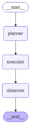
GOAP Execution Graph

The planner discovers a plan, the executor runs each action, and the observer checks progress — replanning automatically if something fails.

from IPython.display import Image, display

graph = GoapGraph(actions=linear_corridor_actions(n_segments=10))
display(Image(graph.compile().get_graph().draw_mermaid_png()))

1. Linear corridor — the simplest planning problem

Ten locations l0, l1, …, l10. Each move_l{i}_to_l{i+1} action has unit cost. The robot starts at l0 and must reach l10.

A* explores the graph forward, finds exactly one path, and returns the sequence of ten moves.

actions = linear_corridor_actions(n_segments=10)

result = GoapGraph(actions=actions).invoke(
    goal=GoalSpec(conditions={"at_l10": True}),
    world_state=linear_corridor_start(n_segments=10),
)

successful = successful_action_names(result)
print(f"Status:        {result['status']}")
print(f"Steps:         {len(successful)}")
print(f"First → Last:  {successful[0]} ... {successful[-1]}")

2. Weighted grid — cost-driven planning

Five locations connected by bidirectional edges with different costs:

              (4)
       A ------------ D
       |              |
    (1)|           (1)|
       |              |
       B --(1)-- C --(1)-- E

Two paths from A to E:

• A → D → E costs 4 + 1 = 5

• A → B → C → E costs 1 + 1 + 1 = 3

A* prefers the longer path because the total cost is lower. This is the core optimality guarantee of A* — minimize g(n), not step count.

result = GoapGraph(actions=weighted_grid_actions()).invoke(
    goal=GoalSpec(conditions={"at_E": True}),
    world_state=weighted_grid_start("A"),
)

successful = successful_action_names(result)
print(f"Status:  {result['status']}")
print(f"Path:    {' → '.join(successful)}")

3. Reverse direction

Edges are bidirectional, so the same cheapest route works in reverse.

result = GoapGraph(actions=weighted_grid_actions()).invoke(
    goal=GoalSpec(conditions={"at_A": True}),
    world_state=weighted_grid_start("E"),
)

successful = successful_action_names(result)
print(f"Status:  {result['status']}")
print(f"Path:    {' → '.join(successful)}")

4. Visualizing the plan

Plan.to_ascii() prints a readable tree that highlights parallel groups (none here — every step depends on the previous one).

from langgoap.planner.astar import plan as astar_plan

plan_obj = astar_plan(
    weighted_grid_start("A"),
    GoalSpec(conditions={"at_E": True}),
    weighted_grid_actions(),
)
print(plan_obj.to_ascii())
print(f"Total cost: {plan_obj.total_cost}")

Summary

• Classical path-finding problems map cleanly to LangGOAP with one boolean per location and one ActionSpec per edge.

• A* finds the cheapest plan, not the shortest — cost-weighted search beats step-count minimization.

• The same A* loop solves corridors, grids, and any other static graph you can describe with preconditions and effects.

Every scenario here is verified by tests/integration/test_robot_navigation.py.